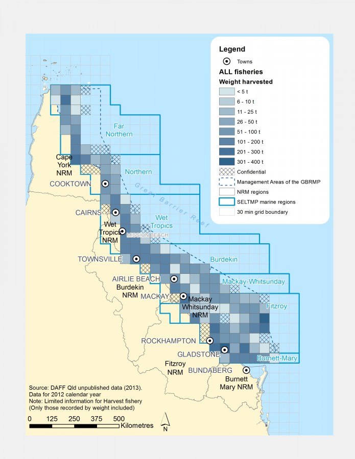
This dataset contains Active Licenses, Effort days, Harvest Weight and GVP for the Queensland commercial harvest, line, net, pot and trawl fisheries. The data is provided on a 30 min grid for locations where there are more than 5 licensed operators. Commercial fishers and charter fishers are required by law to complete daily logbooks. Commercial fishing logbooks are used to record: overall catch, time spent fishing, location where catch was taken and fishing equipment used. This data is then managed by the Department of Agriculture, Fisheries and Forestry (DAFF). This dataset consists of 20 layers (Active Licenses, Effort days, Harvest Weight and GVP) x (commercial harvest, line, net, pot and trawl fisheries). This metadata is not authoritative and was developed as part of the eAtlas project. The shapefiles associated with this dataset were compiled by the SELTMP team.

The low-lying islands of the Torres Strait are vulnerable to climate change and the region faces a range of pressures including a growing population, future climate change, potential pollution as a result of rapid mining and resources development in Papua New Guinea, and increased shipping. Through participatory scenario planning with Torres Strait and PNG communities and stakeholders, informed by integrated ecosystem and climate modelling this project will identify ‘best bet’ strategies to protect livelihoods and achieve sustainable economic development. Tasks include: 1. Identification of key drivers influencing future livelihood pathways in the Torres Strait region. 2. Plausible future scenarios of livelihoods. 3. An agreed typology of livelihoods in the Torres Strait region. 4. An assessment of the adaptive capacity of livelihoods and communities. 5. An assessment of the potential future impacts from drivers on ecosystem services underpinning livelihoods. 6. Identification of the most vulnerable communities and potential case studies for Stage 2 7. Adaptation strategies for these communities. 8. A workshop report summarizing the above for dissemination to all participants.

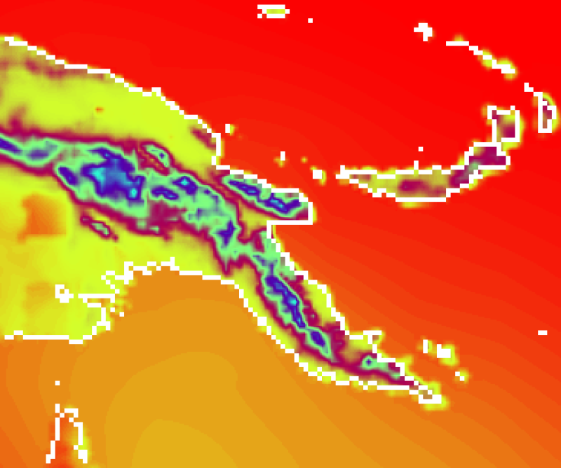
This dataset consists of rasters representing downscaled climate change scenarios (8 km resolution) for the Torres Strait and Papua New Guinea regions for 1990, 2055, 2090. This includes estimated mean surface relative humidity (%), wind speed, rainfall rate (mm per day) and surface temperature (degrees Celsius) estimated from simulated conditions for 1980?1999, 2046-2065 and 2080?2099 time periods. Also included is the relative change of each attribute with respect to 1990. For the past decade the Conformal Cubic Atmospheric Model (CCAM) has been the mainstay of CSIRO dynamical downscaling (McGregor 1996, 2005a, 2005b; McGregor and Dix 2001, 2008). CCAM is an atmospheric GCM formulated on the conformal-cubic grid. CCAM includes a fairly comprehensive set of physical parameterizations. The GFDL parameterizations for long-wave and short-wave radiation (Schwarzkopf and Fels 1991; Lacis and Hansen 1974) are employed, with interactive cloud distributions determined by the liquid and ice-water scheme of Rotstayn (1997). The model employs a stability-dependent boundary layer scheme based on Monin-Obukhov similarity theory (McGregor et al. 1993), together with the non-local treatment of Holtslag and Boville (1993). A canopy scheme is included, as described by Kowalczyk et al. (1994), having six layers for soil temperatures, six layers for soil moisture (solving Richard's equation) and three layers for snow. The cumulus convection scheme uses a mass-flux closure, as described by McGregor (2003), and includes downdrafts, entrainment and detrainment. CCAM is not only used for climate studies (Nguyen et al. 2011), it is also used in a short-range weather forecast system (Landman et al. 2012). Methods: All primary simulations were completed using CSIRO’s global stretched-grid, Conformal Cubic Atmospheric Model (CCAM; McGregor and Dix, 2008) run at 60 km horizontal resolution over the entire globe, while further downscaling to 8 km was conducted for selected partner countries. The CCAM model was chosen for the downscaling because it is a global atmospheric model, so it was possible to bias-adjust the sea-surface temperature in order to improve upon large-scale circulation patterns. In addition, the use of a stretched grid eliminates the problems caused by lateral boundary conditions in limited-area models. The model has been well tested in various model inter-comparisons and in downscaling projects over the Australasian region (Corney et al., 2010). CCAM 60 km Global simulations: These simulations were performed for six host global climate models (CSIRO?Mk3.5, ECHAM/MPI?OM, GFDL-CM2.0, GFDL?CM2.1, MIROC3.2 (medres) and UKMO?HadCM3) that were deemed to have acceptable skill in simulating the climate of the Pacific Climate Change Science Program region. The period 1961-2099 was simulated for the A2 (high) emissions scenario only. In these simulations, the sea-surface temperature bias?adjustment was calculated by computing the monthly average biases of the global models for the 1971-2000 period, relative to the observed climatology, based upon the method of Reynolds (1988). These monthly biases were then subtracted from the global climate model monthly sea-surface temperature output throughout the simulation. This approach preserves the inter- and intra-annual variability and the climate change signal of the host global climate models. CCAM 8 km Global simulations: Due to computational cost, only three of the CCAM 60 km global simulations (those using SSTs from GFDL-CM2.1, UKMO-HadCM3 and ECHAM5) were selected for further downscaling to 8 km. Of the six host models, these three GCM simulations showed a low, middle and high amount of global warming into the future, respectively. A scale-selective digital filter developed by Thatcher and McGregor (2009) was used to impose the broad-scale (scales greater than approximately 500 km) fields of temperature, moisture and winds above pressure-sigma level .9 (about 1 km above the surface) from the 60 km simulations onto the 8 km simulations. Further detail about the methods used in the development of this dataset is provided in: Katzfey, J., Rochester, W., (2012) Downscaled Climate Projections for the Torres Strait Region: 8 km2 results for 2055 and 2090, NERP TE Milestone Report, available: http://nerptropical.edu.au/Project11.1MilestoneReport%E2%80%93May2012%E2%80%93DownscaledClimate Limitations: Climate change projections are inherently uncertain. The future climate will be determined by a combination of factors, including levels of greenhouse gas emissions, unexpected events (e.g. volcanic eruptions), changes in technology and energy use, and sensitivity of the climate system to greenhouse gases, as well as natural variability. Exactly how these factors will unfold is unknown. Climate models have different internal dynamics and parameterisations, and thus respond somewhat differently to the same inputs, producing a range of possible futures. This concern is partly addressed in the current study by selecting CMIP3 GCMs that reproduce current climate reasonably well, then using techniques for bias correction of SSTs that improve their representation in the current climate, but preserve the projected climate change signal and the internal variability. In addition, multi-model means of variables such as temperature and rainfall are assessed to capture the most plausible possible futures. However, the full range of future climate as projected by all GCMs should be considered as well. The best solution is to pick three cases for a given application: the worse case, the best case and the most representative (most evidence) case. This research has revealed some new insights into the potential future climate in Torres Strait, given our current understanding. In assessing the impact of these projections, careful analysis is required. The results presented from this research are only the first step in developing a greater understanding of future climate in Torres Strait. Format: This dataset consists of 5 rasters (in netcdf format) for each attribute (temperature, wind speed, rainfall rate and relative humidity) consisting of 3 time periods (1990, 2055, 2090) plus relative change (1990 to 2055 and 1990 to 2090) for a total of 20 rasters files. References: - Corney SP, Katzfey JF, McGregor JL, Grose MR, White CJ et al (2010) Climate futures for Tasmania: climate modelling technical report. Antarctic Climate and Ecosystems Cooperative Research Centre, Hobart - Katzfey JJ, McGregor JL, Nguyen KC and Thatcher M (2009) Dynamical downscaling techniques: Impacts on regional climate change signals. In MODSIM09 Int. Congress on Modelling and Simulation, www.mssanz.org.au/modsim09 13:2377-2383 - McGregor JL (2005) C-CAM: Geometric aspects and dynamical formulation. CSIRO Atmospheric Research Technical Paper 43 - McGregor JL and Dix MR (2008) An updated description of the Conformal-Cubic Atmospheric Model. In: “High Resolution Simulation of the Atmosphere and Ocean”, Hamilton K and Ohfuchi W (Eds), Springer, 51–76 - Nguyen KC, Katzfey JJ, McGregor JL (2011) Global 60 km simulations with CCAM: evaluation over the tropics. Clim Dyn online first. doi:10.?1007/?s00382-011-1197-8 - Reynolds RW, Smith TM, Liu C, Chelton DB, Casey KS and Schlax MG (2007) Daily high-resolution blended analyses for sea surface temperature. J Climate 20:5473-5496

This very large study is published in Pitcher et al. (2007). Its purpose was to quantify patterns in seabed biodiversity and inter-reefal environmental conditions throughout the GBR. The study had three aims: (1) Assessment of seabed biodiversity on the continental shelf of the Great Barrier Reef World Heritage Area, and assessment of the use of biophysical data as environmental correlates of biodiversity and benthic communities; (2) Mapping bycatch and seabed benthos assemblages in the GBR Region for environmental risk assessment and sustainable management of the Queensland East Coast Trawl Fishery, and (3) Assessment of the performance of acoustic remote sensing for seabed mapping and as a surrogate for biodiversity on the continental shelf of the GBR. It contains several large data sets, based on >600 km of towed video, ~100,000 photos, 1150 baited remote underwater videos, echograms, ~14,000 benthic samples, ~4,000 seabed fish samples, and ~1,200 sediment samples. The eAtlas has processed the Towed video data into a shapefile [1 MB] for dataset visualisation. This processing was done by combining the start and end tow events from the VESSEL_TASKS_ALL table to create a shapefile (GBR_CSIRO-AIMS_Seabed-biodiversity-2003-2006_DropCam.shp) and CSV (GBR_CSIRO-AIMS_Seabed-biodiversity-2003-2006_DropCam.csv) with a line feature for each tow. The information from tables VESSEL_VIDEO_BIOHABITAT and VESSEL_VIDEO_SUBSTRATUM were added as attributes of the line features based on the matching SITE_ID. Format: The processed data from this study is stored in an Access Database (77 MB). The eAtlas summarised the tow video data into a shapefile [1MB] and CSV files (290 KB). Note the attribute names in the shapefile were truncated to 10 characters due to the limitation of shapfiles. These names are provided in the Data Dictionary below. Data Dictionary: The following are descriptions of all the attributed in the tables of the Access Database. Each section corresponds to a table in the database. SITE_DATA: - SITE_ID: site ID number - GRD_ID: 0.01 degree gridcell ID number - GRD_LAT: latitude centre of GRD_ID grid cell (GDA94) - GRD_LON: longitude centre of GRD_ID grid cell (GDA94) - STRATUM_ID: biophysical stratification membership number - SNDR_DEPTH: site echosounder depth (metres) - GBR_ASPECT: derived aspect from GBRMPA 15 second bathymetry - GA_CRBNT: % carbonate of sediment samples, processed by Geoscience Australia - GA_GRAVEL: % gravel grainsize fraction of sediment samples, processed by Geoscience Australia - GA_SAND: % sand grainsize fraction of sediment samples, processed by Geoscience Australia - GA_MUD: % mud grainsize fraction of sediment samples, processed by Geoscience Australia VESSEL_TASKS_ALL: - SITE_ID: site ID number - VESSEL_ID: vessel ID code: LB=Lady Basten (AIMS), GM=Gwendoline May (QDPI) - DTTM_EST: date/time (EST) of task event on vessels - LATITUDE: latitude of task event, decimal degrees - LONGITUDE: longitude of task event, decimal degrees - DEPTH: depth of task event (m), recorded from vessel echosounder - EVENT_1: drop camera deployment & recovery task events - EVENT_2: drop camera transect start & end task events - EVENT_3: 1.5m epibenthic sled tow start & end task events - EVENT_4: BRUVS deployment task events - EVENT_5: research trawl (8 fathom Florida Flyer) tow start & end task events VESSEL_TASKS_BRUVS: - SITE_ID: site ID number - VESSEL_ID: vessel ID code: LB=Lady Basten (AIMS) - DTTM_EST: date/time (EST) of BRUVS deployment event on vessel - LATITUDE: latitude of BRUVS deployment event, decimal degrees - LONGITUDE: longitude of BRUVS deployment event, decimal degrees - DEPTH: depth of BRUVS deployment event (m), recorded from vessel echosounder - BRUV_ID: ID number of BRUVS deployed VESSEL_TASKS_DROPCAM: - SITE_ID: site ID number - VESSEL_ID: vessel ID code: LB=Lady Basten (AIMS) - DTTM_EST: date/time (EST) of DROPCAM transect start event on vessel - LATITUDE: latitude of DROPCAM transect start event, decimal degrees - LONGITUDE: longitude of DROPCAM transect start event, decimal degrees - DEPTH: depth of DROPCAM transect start event (m), recorded from vessel echosounder - DURATION: duration of DROPCAM transect tow (minutes) - LENGTH: length of DROPCAM transect tow (metres) VESSEL_TASKS_SAMPLING: - SITE_ID: site ID number - VESSEL_ID: vessel ID code: LB=Lady Basten (=>SLED), GM=Gwendoline May (=>TRAWL) - DTTM_EST: date/time (EST) of sampling tow start event on vessel - LATITUDE: latitude of sampling tow start event, decimal degrees - LONGITUDE: longitude of sampling tow start event, decimal degrees - DEPTH: depth of sampling tow start event (m), recorded from vessel echosounder - DURATION: duration of sampling tow (minutes) - LENGTH: length of sampling tow (metres) - AREA_HA: swept area of sampling tow (hectares) VESSEL_SAMPLES: - SITE_ID: site ID number - SAMPLE_ID: sample ID number - VESSEL_ID: vessel ID code: LB=Lady Basten (AIMS), GM=Gwendoline May (QDPI) - SAMPLE_DATE: sampling date (EST) - CLASS: preservation class for sampled biota - DATA_RECORDER: name of data recorder on vessel - CONTAINER_ID: container ID number for storage of samples preserved on vessel - LABORATORY: destination laboratory for sorting of specimens - PRESERVATION: type of preservation - SAMPLE_TOTAL_WT: total weight of sample before any sub-sampling - SAMPLE_RETAINED_WT: weight of sample after any sub-sampling, retained for lab sorting - COMMENTS: comments LAB_SPECIMEN_TAXA: - OTU_ID: operational taxonomic unit ID number, nominal species equivalent - KINGDOM: taxonomic kingdom name - PHYLUM: taxonomic phylum name - CLASS: taxonomic class name - ORDR: taxonomic order name - FAMILY: taxonomic family name - GENUS: taxonomic genus name - SPECIES: taxonomic species name, if identified - otherwise alpha taxonomy applies - DESCRIPTION: specimen description - LOCATION: location of OTU, note synonymous OTUs may reside in other labs - SITE_ID: site ID number - SAMPLE_ID: sample ID number - OTU_ID: operational taxonomic unit ID number, nominal species equivalent - LAB_WT: weight (g) of specimens where measured (negative = not weighed) - LAB_CNT: count of specimens where distinct (negative = not countable) BRUVS_SPECIES_CAAB: - CAAB_CODE: species Codes for Australian Aquatic Biota www.marine.csiro.au/caab/ - KINGDOM: taxonomic kingdom name - PHYLUM: taxonomic phylum name - CLASS: taxonomic class name - ORDER: taxonomic order name - FAMILY: taxonomic family name - GENUS: taxonomic genus name - SPECIES: taxonomic species name, if identified BRUVS_maxN_DATA: - SITE_ID: site ID number - BRUV_NUM: BRUV Station ID number within Site - CAAB_CODE: species Codes for Australian Aquatic Biota www.marine.csiro.au/caab/ - MAXN: maximum count of species in any single video frame recorded at station VESSEL_VIDEO_SUBSTRATUM: Note the names in brackets correspond to the attribute name in the shapefile. - SITE_ID(SITE_ID): site ID number - SoftMud(SoftMud): percentage of Soft Mud observed along video transect - Silt(Sandy-Mud)(Silt): percentage of Silt (Sandy-Mud) observed along video transect - Sand(Sand): percentage of Sand observed along video transect - CoarseSand(CoarseSand): percentage of Coarse Sand observed along video transect - SandWaves/Dunes(SandDunes): percentage of Sand Waves / Dunes observed along video transect - Rubble(5-50mm)(Rubble): percentage of Rubble (5-50mm) observed along video transect - Stones(50-250mm)(Stones): percentage of Stones (50-250mm) observed along video transect - Rocks(>250mm)(Rocks): percentage of Rocks (>250mm) observed along video transect - Bedrock/Reef(Bedrock): percentage of Bedrock / Reef observed along video transect VESSEL_VIDEO_BIOHABITAT: Note the names in brackets correspond to the attribute name in the shapefile. - SITE_ID(SITE_ID): site ID number - NoBiohabitat(NoBiohabit): percentage of seab with No Biogenic habitat observed along video transect - Bioturbated(Bioturbate): percentage of Bioturbated seabed observed along video transect - AlcyonariansSparse(AlcyonSpar): percentage of Sparse Alcyonarians observed along video transect - AlcyonariansMedium(AlcyonMed): percentage of Medium Alcyonarians observed along video transect - AlcyonariansDense(AlcyonDens): percentage of Dense Alcyonarians observed along video transect - WhipGardenSparse(WhipGaSpar): percentage of Sparse Whip Garden observed along video transect - WhipGardenMedium(WhipGaMed): percentage of Medium Whip Garden observed along video transect - WhipGardenDense(WhipGaDens): percentage of Dense Whip Garden observed along video transect - GorgonianGardenSparse(GorgonSpar): percentage of Sparse Gorgonian Garden observed along video transect - GorgonianGardenMedium(GorgonMed): percentage of Medium Gorgonian Garden observed along video transect - GorgonianGardenDense(GorgonDens): percentage of Dense Gorgonian Garden observed along video transect - SpongeGardenSparse(SpongeSpar): percentage of Sparse Sponge Garden observed along video transect - SpongeGardenMedium(SpongeMed): percentage of Medium Sponge Garden observed along video transect - SpongeGardenDense(SpongeDens): percentage of Dense Sponge Garden observed along video transect - HardCoralGardenSparse(HardCoSpar): percentage of Sparse Hard Coral Garden observed along video transect - HardCoralGardenMedium(HardCoMed): percentage of Medium Hard Coral Garden observed along video transect - HardCoralGardenDense(HardCoDens): percentage of Dense Hard Coral Garden observed along video transect - LiveReefCorals(LiveReefCo): percentage of Live Reef Corals observed along video transect - Flora(Flora): percentage of Flora observed along video transect - Algae(Algae): percentage of Algae observed along video transect - Halimeda(Halimeda): percentage of Halimeda observed along video transect - Caulerpa(Caulerpa): percentage of Caulerpa observed along video transect - Seagrass(Seagrass): percentage of Seagrass observed along video transect - BivalveShellBeds(BivalShBed): percentage of Bivalve Shell Beds observed along video transect - SquidEggs(SquidEggs): percentage of Squid Eggs observed along video transect - TubePolychaeteBeds(TubePolBed): percentage of Tube Polychaete Beds observed along video transect LAB_VIDEO_HABITAT_DATA: - SITE_ID: site ID number - FRAME_NO: transect video segment frame number - HABITAT_TYPE: habitat category type: Biological, Sediment, Physical - FEATURE: habitat feature descripor within category type - DESCRIPTOR1: first descriptor of habitat feature, if applicable - DESCRIPTOR2: secondary descriptor of feature, if applicable - PERCENT_COVER: percent cover of frame by feature of given descriptor - VERTICAL_SCALE: vertical scale of feature (cm), if recorded - HORIZONTAL_SCALE: horizontal scale of feature (cm), if recorded Reference: Pitcher, C.R., Doherty, P., Arnold, P., Hooper, J., Gribble, N., Bartlett, C., Browne, M., Campbell, N., Cannard, T., Cappo, M., Carini, G., Chalmers, S., Cheers, S., Chetwynd, D., Colefax, A., Coles, R., Cook, S., Davie, P., De'ath, G., Devereux, D., Done, B., Donovan, T., Ehrke, B., Ellis, N., Ericson, G., Fellegara, I., Forcey, K., Furey, M., Gledhill, D., Good, N., Gordon, S., Haywood, M., Hendriks, P., Jacobsen, I., Johnson, J., Jones, M., Kinninmoth, S., Kistle, S., Last, P., Leite, A., Marks, S., McLeod, I., Oczkowicz, S., Robinson, M., Rose, C., Seabright, D., Sheils, J., Sherlock, M., Skelton, P., Smith, D., Smith, G., Speare, P., Stowar, M., Strickland, C., Van der Geest, C., Venables, W., Walsh, C., Wassenberg, T., Welna, A., Yearsley, G. (2007). Seabed Biodiversity on the Continental Shelf of the Great Barrier Reef World Heritage Area. AIMS/CSIRO/QM/QDPI CRC Reef Research Task Final Report. 320 pp. Data Location: This dataset is saved in the eAtlas enduring data repository at: data\custodian\2009-2019-other\GBR_CSIRO-AIMS_Seabed-biodiversity-2003-2006

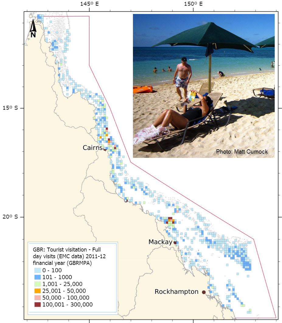
This dataset shows the spatial distribution of the number of visitors to the Great Barrier Reef Marine Park based on visitation rates collected from the Environmental Management Charge (EMC) managed by GBRMPA. The spatial information has been quantised into a 0.1 degree grid size. This data only represents visitors to the Great Barrier Reef who used commercial tourist operations. Data is collected and updated quarterly following receipt of Environmental Management Charge returns from tourism operators. This dataset is a set of annual snapshots of this monthly data. The count of visitor days to the Marine Park is calculated where passengers undertake a visit as follows: Full day visits: A day trip of more than three hours is recorded as a full day visit. Overnight trips are recorded as multiple full days, for example, a stay of two-days and one night is counted as two full day visits. Part day visits: Where the trip is less than three hours. The first day of a trip entering the Marine Park after 5 pm. The last day of a trip leaving the Marine Park before 6 am. Exempt visits are passengers who are not required to pay the Environmental Management Charge (EMC), for example: young children who are free-of-charge, trade familiarisation passengers who are free-of-charge, passengers for whom another operator has already paid EMC on that day and the fourth and subsequent days for passengers on extended charters. This metadata is not authoritative and was developed for documenting layers on the eAtlas. This dataset was supplied by the SELTMP team (http://seltmp.eatlas.org.au). Please contact the SELTMP of GBRMPA for further information. Format: This dataset consists of two shapefiles, one for the 2010-2011 financial year and one for the 2011-2012 financial year.

Long-term social and economic monitoring helps reef managers understand the current status of marine park users, industries and communities. It also helps build a picture of how industries and communities are likely to respond and cope with changes associated with environmental degradation, climate change, regulatory frameworks, and changes in culture. It can also assist in evaluating the effectiveness of management interventions.This project will establish and collect a unique data set that documents long-term social and economic trends in communities and users of the Great Barrier Reef (GBR). In 2011-12 a number of existing datasets were collated and relevant information extracted. Additionally data gaps were identified, which then formed the primary survey questions. In 2012-13 and 2013-14 primary data will be collected via surveys conducted on mini iPads from Bundaberg to Cooktown. Outcomes of this project include: * Providing GBR management and industries with better access to social and economic information necessary for planning purposes. * Strong liaison with GBR stakeholders on the social and economic status of the region. * An annual snapshot of the social and economic indicators for the entire GBR region.